The measurement
This thesis presents the first measurement of the longitudinal polarisation states of one or both bosons in processes, using the data recorded by the ATLAS experiment during the full Run-2 of the LHC, corresponding to an integrated luminosity of at a centre-of-mass energy of , combined with the first part of Run-3, corresponding to at .
The polarisation being only a statistical property of the bosons, it is not possible to measure it directly via an observable, but it can be inferred from the angular distribution of the decay products of the bosons. Three distinct measurements are considered: both bosons longitudinally polarised (), the most challenging, with only of the total event yield; only the boson longitudinally polarised (); and only the boson longitudinally polarised ().
Signal-background and polarisation DNNs
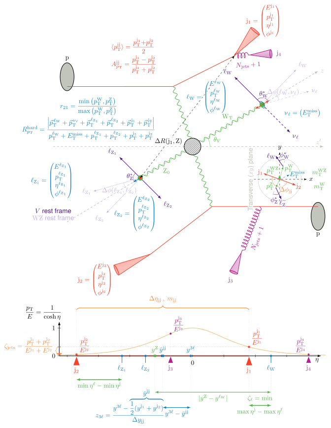
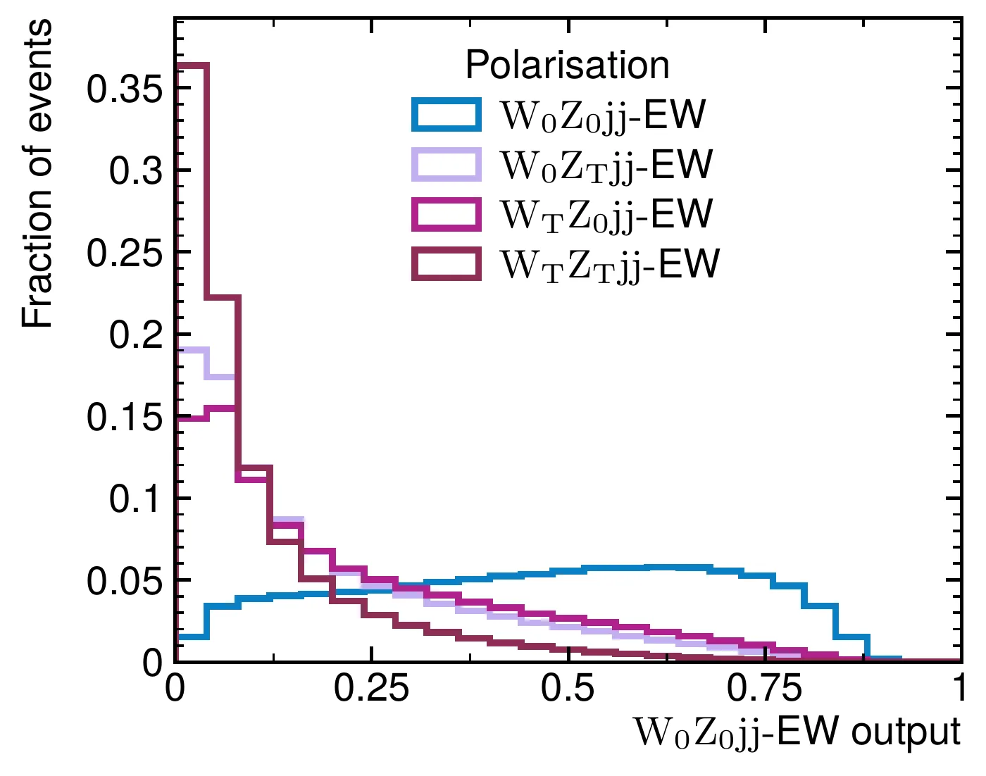
Deep neural networks are trained to separate events from the background and then to disentangle the polarisation states. All DNNs are feed-forward fully connected NNs with a ReLU activation function for the hidden layers, and a dropout layer between the hidden layers to prevent overfitting. The hyperparameters of each DNN are optimised using a Bayesian optimisation, and the networks are trained in five folds, so that each event entering the final template is evaluated by a DNN that was not trained on that event.
More: constraints on the DNN architecture
The DNN architecture was subject to constraints due to portability to the analysis framework in C++ but also to Fortran, in which MoCaNLO is written. MoCaNLO is a fixed-order integrator, not an event generator, so the non-negligible NLO EW correction to the measured observable can only be obtained by evaluating the DNNs and the Voronoi binning inside the integration, event by event. More elaborate architectures could therefore not be used. However, a study comparing the present setup to an adaptation of the transformer using the GN2 network developed for jet tagging was carried out. No improvement was observed with respect to the present methods.
Two-dimensional template
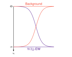
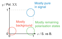
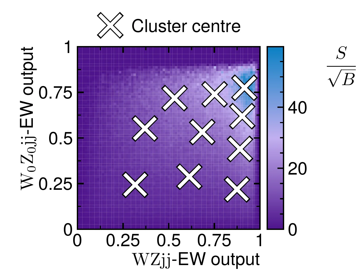
The final discriminant planes are built using the output of the S. vs B. DNN with the output (giving us the probability of having the signal) on the -axis and the output of one of the polarisation DNNs on the -axis (giving us the probability of having the desired polarisation state). The signal is expected to be concentrated in the top right corner of the plane, while the background is expected to be concentrated in the bottom left corner. The bottom right corner is expected to be the signal but with the non-targeted polarisation states.
Voronoi-based binning
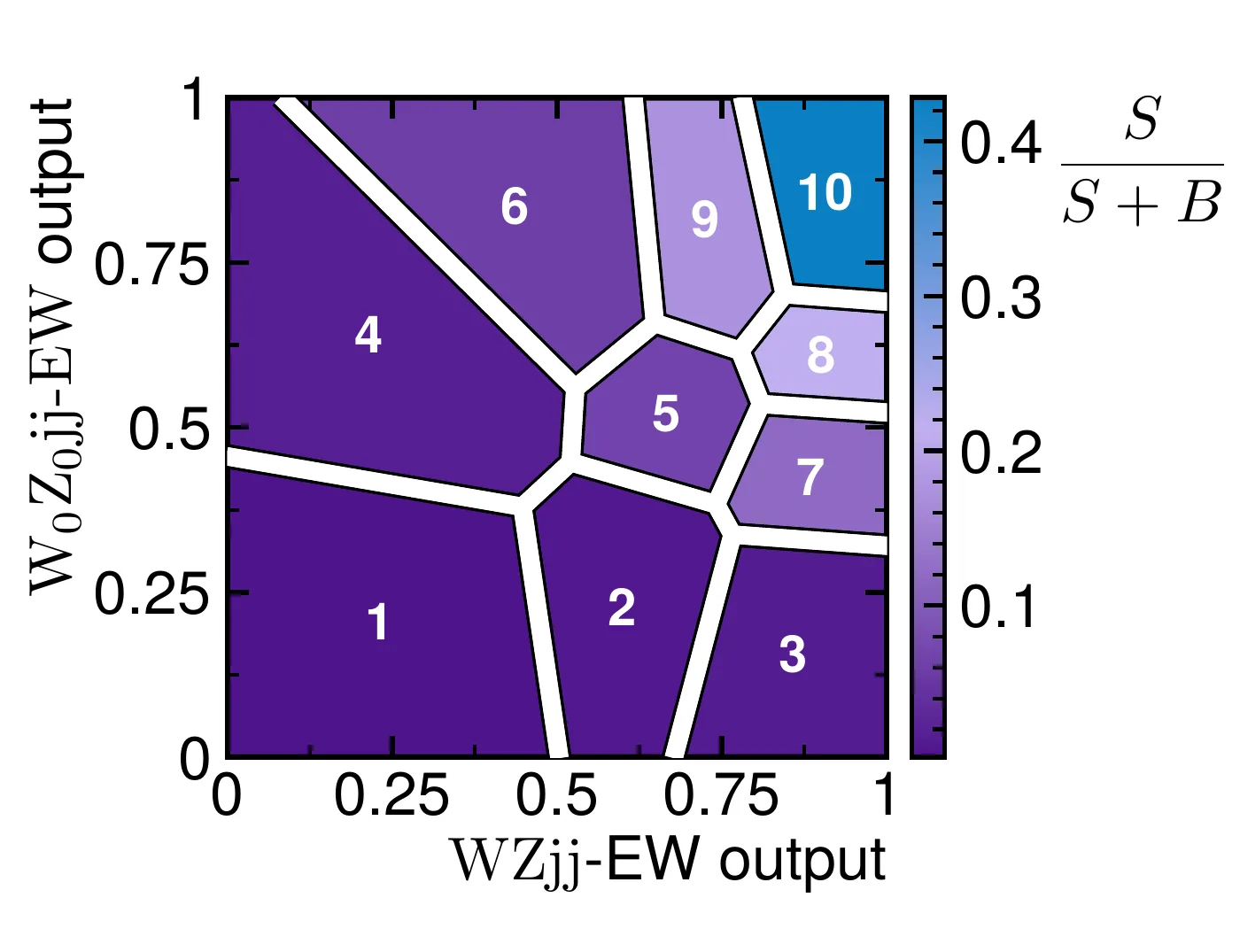
The retained method works in two steps. The first part is to form a 2D histogram showing the ratio of signal over the square root of the background, , using a fine binning (here bins). Then we compute the -means clusters on the signal only, using the value in each bin as a per-event weight, so that signal-rich bins with a large exert a stronger pull on the cluster centres. In this way the algorithm concentrates the centres in the regions of the discriminant plane with the highest signal significance.
The second step then consists of applying a Voronoi binning using the cluster centres as seeds: each Voronoi region is the set of points that are closer to a particular cluster centre than to any other cluster centre. The number of clusters is set to , presenting a good compromise between having enough bins to exploit the DNN discrimination power and keeping a reasonable number of bins to avoid large statistical uncertainty in each bin. The bins are ordered by increasing .
More: comparison with rectangular binnings
This new method yields a clear improvement, with an increase in expected significance of a few percent over the best rectangular configuration and up to over the worst one, depending on the measured polarisation state. At fixed bin multiplicity, the -bin Voronoi tessellation systematically matches or exceeds the best rectangular configuration. The rectangular results also depend strongly on the choice of axis ordering, with the and layouts differing by up to in expected significance, while the Voronoi binning naturally avoids this arbitrariness. It also tackles the reduced output range of the Pol. DNN output, as the bins are not rectangular and can be adapted to the shape of the distribution.
Binned maximum-likelihood fit
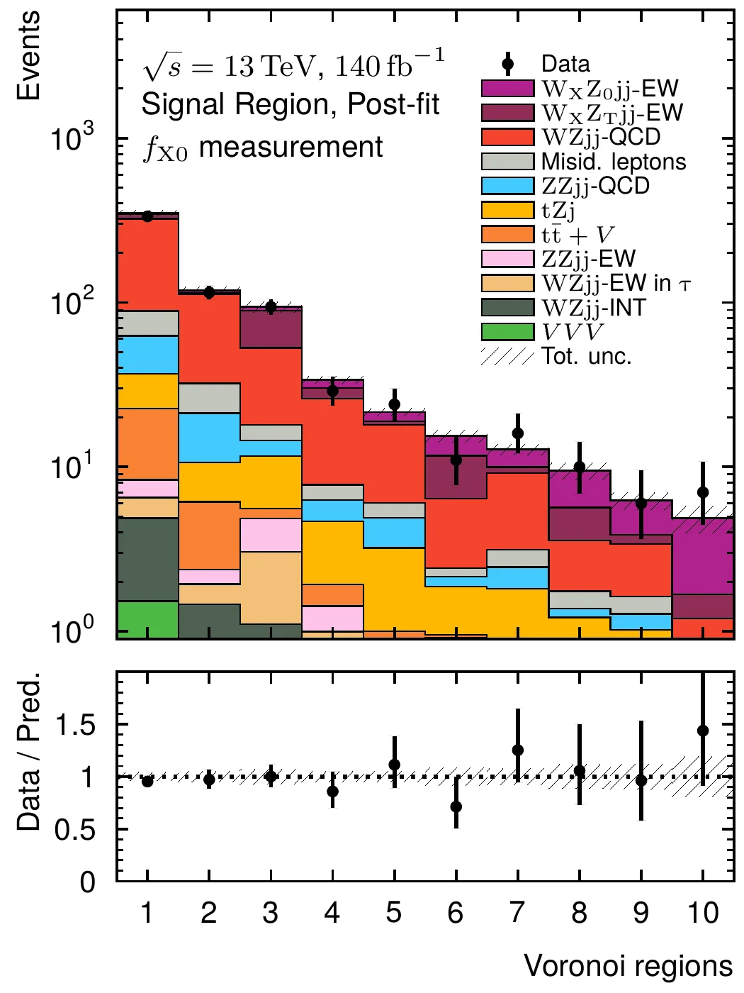
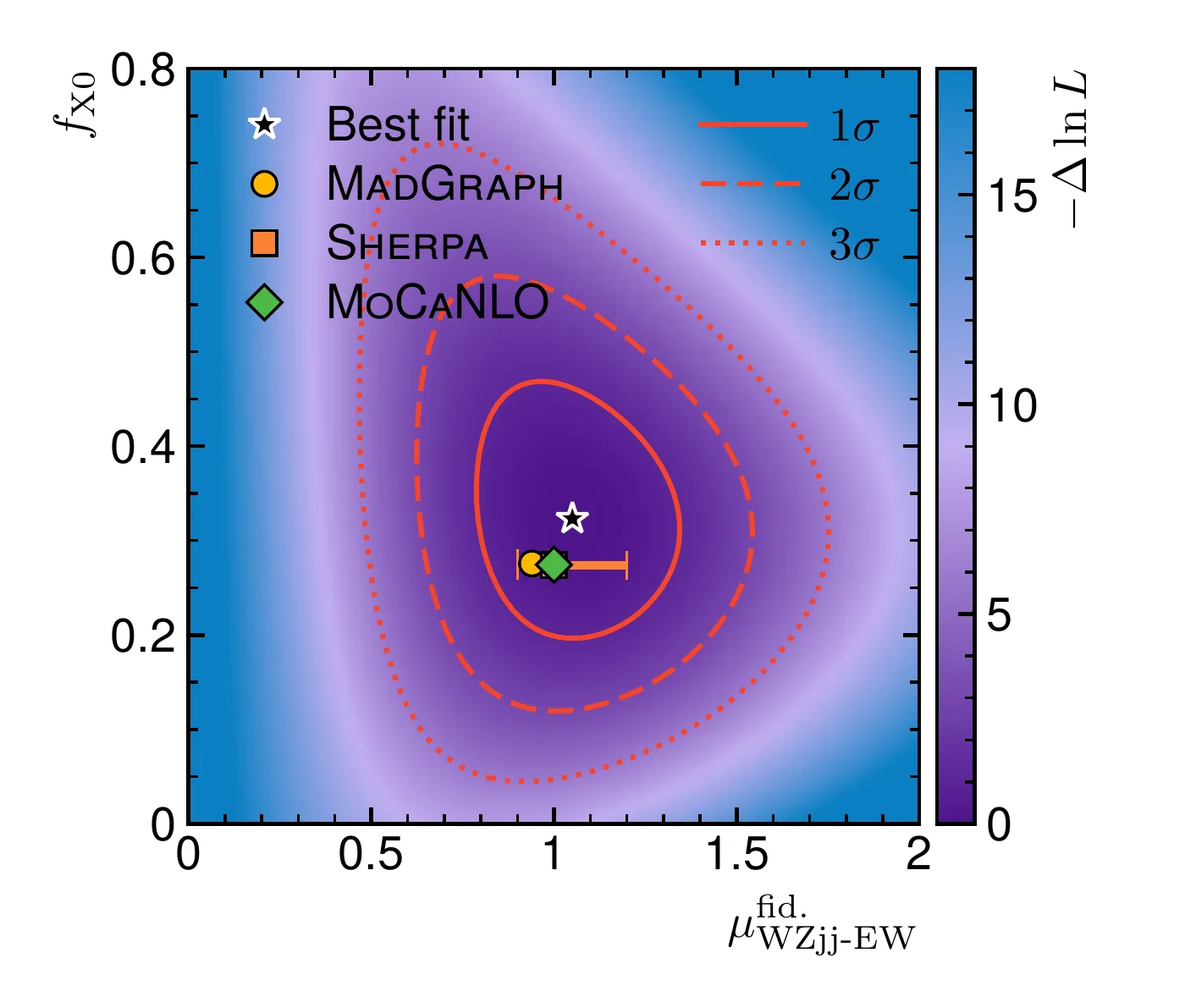
The unrolled Voronoi templates of the signal region are fitted together with two control regions, with a binned maximum-likelihood fit. The parameters of interest are the polarisation fraction and the fiducial signal strength , which gives the fiducial cross-section with the total number of events in the fiducial phase-space and the integrated luminosity; the factor accounts for the four decay channels , , , and . The polarised and non-polarised components are then normalised by so that only and float freely.
Results
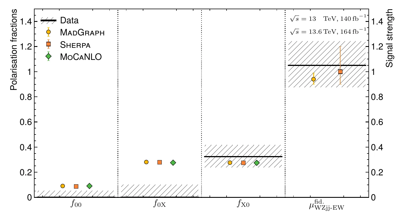
The fraction of events in which the boson is longitudinally polarised regardless of the polarisation of the boson is measured to be , for a prediction of , with an observed (expected) significance of () standard deviations, providing the first evidence for longitudinally polarised -boson states in events. The fraction of events in which both bosons are longitudinally polarised is measured to be , for a Standard Model prediction of , and the fraction in which the boson is longitudinally polarised to be , for a prediction of . Upper limits at confidence level are set at ( expected) and ( expected), respectively. The signal strength of the process is found to be , and its fiducial cross-section per lepton flavour is reported at for the first time:
More: two-dimensional likelihood scan
These measurements are statistically limited, and will benefit from the High-Luminosity LHC and from the replacement of the current tracking detector with the new Inner Tracker, extending the absolute pseudorapidity coverage from to .